Getting started
What you need before you can generate anything, the parts of the main window, and the order the work happens in.
Three things have to be in place before the application can place a single module table: the application installed on a Windows PC, active access for this device, and one file describing where the plant goes. Every other input ships with a working default, so a first run needs almost none of them.
The work happens on your own machine. The steps that reach the internet are verifying this device's access, fetching weather data for the energy estimate, fetching elevation data for the terrain check, and the aerial photograph behind the layout — the last three are optional.
Before you start
| What you need | Why | Where |
|---|---|---|
| The application | A Windows PC, installed from the Microsoft Store | Install on Windows |
| This device activated | The application opens without it, but Generate Layout and the exports are blocked until access is active | Activate your licence |
| A boundary file | The plant boundary, and any water bodies, obstructions and transmission lines inside it | Boundary files |
Access is tied to this computer by a Device ID — the same value shown at Settings ▸ System ▸ About ▸ Device ID. There is no licence file to install, copy, back up or keep safe: status is verified online with the server. Open Help ▸ License / Subscription… and click Get Free Access to activate this device — see Activate your licence.
The boundary file can be a Google Earth file (.kmz or .kml), a CAD drawing
(.dxf), or a raster image with a scale you supply. A Google Earth
file is the recommended input, because it carries geographic position and the
site's features in one place. For a CAD drawing or an image you are asked
where it sits — by a CAD drawing's own UTM coordinates, or by the latitude and
longitude of the site's centre. Layout only still generates the layout,
but energy cannot be calculated.
Two decisions at launch
Every launch opens the SolarLayout · New design window before the main window. Two segmented controls ask how the plant is mounted — Fixed tilt or Single-axis tracker — and how it is wired — String inverter or Central inverter. A card under them summarises the combination, and Continue opens the main window for it. The choice controls which input cards you see and how the plant is put together; a different design later means a second window, not a switch. See Choosing a design mode.
The main window
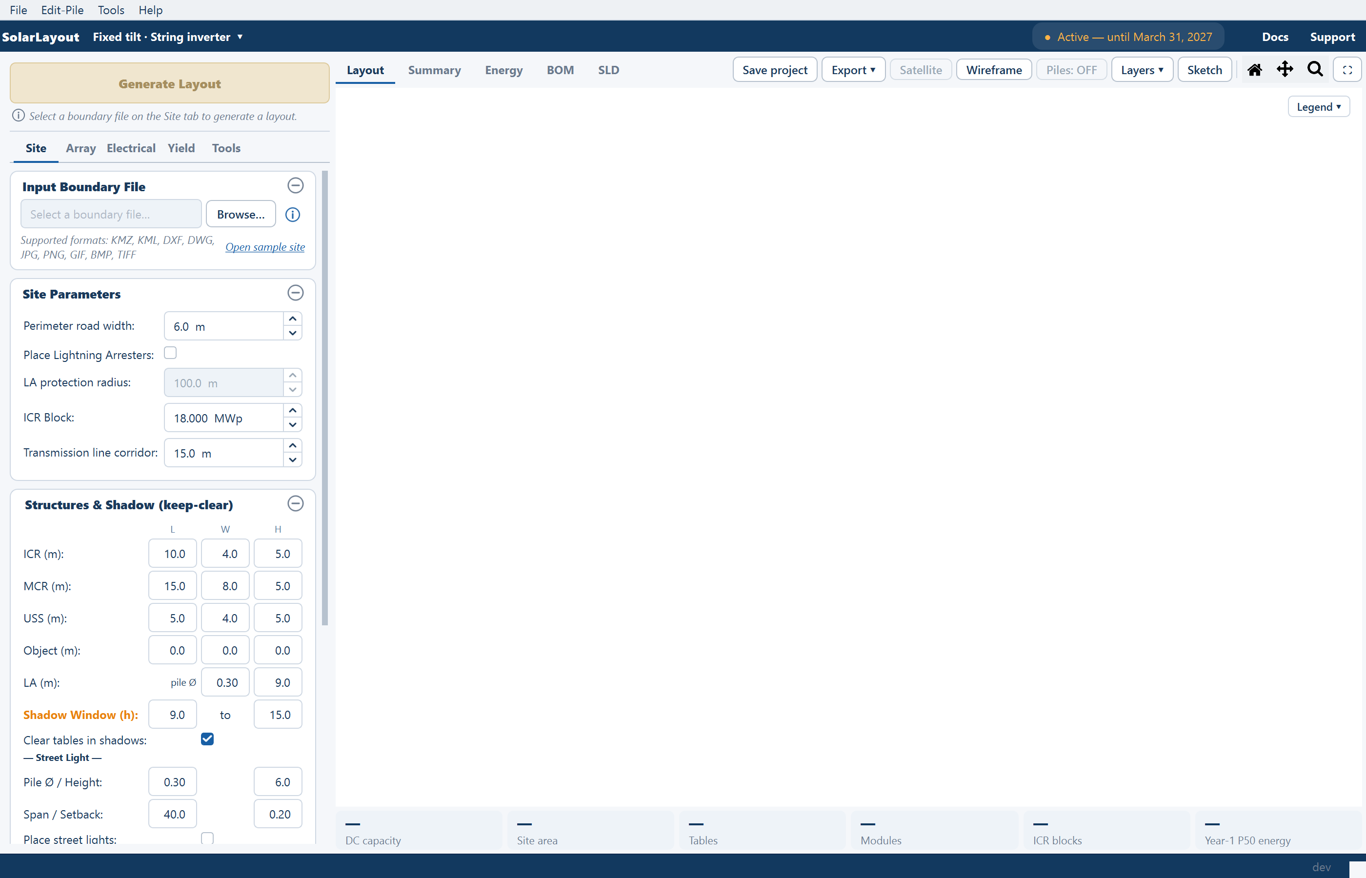
| Region | What it is |
|---|---|
| Menu bar | File, Edit-Pile, Tools and Help: projects, the pile editor, the robot count from a DXF and the earthing design, the in-app guide and the licence window. |
| The ribbon | The SolarLayout brand; the design chip naming this window's design, which opens another window for a different one; the access chip; and the Docs and Support buttons. |
| Generate Layout, pinned at the top of the left column | The gold button (F5), with a hint line under it that says why it is disabled — "Select a boundary file on the Site tab to generate a layout." until a file is chosen. While an input differs from the last run it reads Regenerate Layout. |
| The five stage tabs, under it | Site · Array · Electrical · Yield · Tools — every design input, as collapsible cards. |
| The view tabs, across the top of the right side | Layout · Summary · Energy · BOM · SLD (Ctrl+1 to Ctrl+5), with the current view's tools to their right. |
| The view | The drawing, the summary sheet, the energy result, the bill of materials or the diagram — one at a time, filling the area. |
| The plant chips, under the view | One row of plant totals — DC capacity, site area, tables, modules, ICR blocks, year-one energy — shown in every view, led by an Out of date or Design warnings chip when either applies. |
| Status bar | Progress and result messages on the left; the cursor position and the application version on the right. The position is in UTM metres, or in the drawing's own coordinates for a CAD drawing or image placed by latitude and longitude, or laid out only. |
The main window walks through each region.
The stage tabs
The tabs run in the order you would normally work through them. Two of the Array cards depend on the mounting you chose at launch, and the names of two Electrical cards depend on the inverter.
| Tab | What it holds |
|---|---|
| Site | Input Boundary File — the file, a Browse… button, an ⓘ button for the preparation guide and, while empty, an Open sample site link; then Site Parameters, Structures & Shadow (keep-clear) and Topography (slope-aware exclusion) |
| Array | A read-only MOUNTING chip, Module Specifications, then MMS-Table Configuration and Spacing & Tilt on a fixed-tilt design or Tracker Configuration on a tracker |
| Electrical | String Inverter (or SMB – String Monitoring Box), ACCB & Transformer (Transformer on a central design) and Cables |
| Yield | Run Energy Calculation and Energy Yield |
| Tools | Obstructions, Main Control Room & Objects and Studies — the buttons are greyed out until a layout exists, except Robot count from DXF… |
The views and their tools
Beside the view tabs sit Save project and Export ▾ in every view. On the Layout view they are joined by Satellite, Wireframe, Piles, a Layers ▾ popover, Sketch, the Home, Pan and Zoom tools and an expand button; on Summary and Energy by Copy and Open in window.
The Layers ▾ popover holds the drawing's ON/OFF rows. Plant layout and Plant totals start on; Legend, Lightning arresters, ICR blocks, the three cable rows and Contour / terrain start off, so a first layout is drawn as the placement alone even where those figures have been computed. Views, layers and tools covers every row and tool.
How the work flows
| Stage | What you do | More |
|---|---|---|
| 1. Load a boundary | On the Site tab, point Browse… at your file, or click Open sample site. The boundaries, obstacles, water bodies and line features are read from it. | Boundary files |
| 2. Set inputs, or accept the defaults | Change what your design fixes — module, table size, road width, capacity block — and leave the rest. | Every parameter and its default |
| 3. Generate the layout | Click Generate Layout. Tables, control rooms, inverters and arresters are placed, the plant chips fill in, and the Tools tab's buttons come on. | Your first layout |
| 4. Refine | Change an input and generate again — results show they are out of date until you do — or edit the layout by hand: move, add and delete units, draw obstructions, drag a control room. | Editing by hand |
| 5. Calculate energy | Optional. Fetches irradiance for the site and reports year-one and lifetime generation against a performance ratio you control, on the Energy view. | How yield is calculated |
| 6. Build the diagram and the materials list | Auto-build a single-line diagram from the plant's own counts on the SLD view, and rebuild the bill of materials from the layout on the BOM view. | Single-line diagram |
| 7. Export or save | From Export ▾: the Word project report, a Google Earth file, a layered CAD drawing, ICR-block drawings as DXF or PDF, the cable schedule, the plot as an image — or Save project to reopen later. | The project report |
Steps 3 to 6 are not one-way. Generating again after a change is the normal way to work. The obstructions, main control room, objects and annotations you placed are carried onto the new layout; hand-placed tables and hand-drawn cable trenches are not, so draw trenches after the last Generate.
Defaults mean a first run needs almost nothing
The boundary file is the only input with no default. Everything else is pre-filled with a value a utility-scale design would recognise, so you can generate a complete layout on your first run and then decide what to change.
| Input | Default |
|---|---|
| Module | 2.38 m × 1.13 m, 610 Wp, monofacial |
| Table | Portrait, 28 modules per row, 2 rows per table |
| Perimeter road width | 6.0 m |
| Control-room capacity block | 18.000 MWp |
| Tilt angle and row pitch | Derived from the site latitude |
| Cable calculation | Off |
Tilt and row pitch deserve a note: with both override boxes left unticked, the application derives the tilt from the site latitude and the row pitch from the no-shading spacing at winter-solstice solar noon. After a run, both derived values are reported on the Array tab and pre-filled into the override boxes, so you can see what was chosen before deciding to fix it yourself. Auto-calculated values are marked with an asterisk in the Summary view.
Cable calculation is off by default, and worth leaving off for a first run. It is the slow step on a large or complex layout, and the counts of inverters and monitoring boxes are computed either way — only the cable rows read as not computed.
Where to go next
Your first layout
Boundary file in, finished layout, energy estimate and project report out
The main window
The ribbon, the stage tabs and the status bar
Views, layers and tools
The five views, the Layers popover and the plant chips
Choosing a design mode
What the New design window asks and what each answer changes
What SolarLayout Desktop does
A Windows application that turns a site boundary into a complete PV plant design — layout, energy yield, diagrams, and the drawings your team builds from.
Install on Windows
Install from the Microsoft Store, launch the application for the first time, and choose a design mode.