Your first analysis
A complete first run — project type, generation profile, peak window, Simulate, and reading the result.
This walkthrough runs one analysis from an empty window to an exported report, changing as little as possible along the way. It assumes the default project type, 3. Solar + Wind + BESS, and a generation profile you already have as a CSV.
Pick a project type
On the 📂 Data tab, a radio group chooses the plant's topology. The default, ticked at launch, is 3. Solar + Wind + BESS. Leave it there for this run — see Choosing a project type for what the other three change.
Below the radio group, a Peak-Shift dispatch checkbox is off by default. Leave it off too; it changes how the battery is scheduled, covered on the same page.
Load a generation profile
Still on the 📂 Data tab: click Browse…, pick your file, then click Load & Preview CSV. The status line beneath starts No file loaded. and is replaced by a summary once the file reads correctly.
The file needs three columns — a datetime column, one solar generation column and one wind generation column, each value per‑1‑MW‑installed between 0 and 1. Column headers don't have to match exactly: the app looks for common keywords in the name (solar/pv/sun for one, wind/wtg/turbine for the other) and falls back to the first and second numeric columns if none match; the datetime column is found the same way, or built for you if the file doesn't have one. 15-minute, 30-minute and hourly rows are all accepted — the app detects which one your file uses automatically, then upsamples anything coarser than 15 minutes to that base by repeating each row across its sub-intervals.
If you picked 4. Standalone BESS (grid-charged) in the previous step, skip this step entirely — its generation-profile loader is disabled, and a full year's 15-minute calendar is built for you instead.
Set the peak window
On the ⏰ Peak tab, 24 hourly checkboxes split the day into Peak and Off-Peak. On Peak hours the battery discharges first, to help meet the Contracted Capacity (CC) — the firm load the plant is obligated to serve, set on the 📐 Sizing tab — and any excess generation then charges it. On Off-Peak hours the battery charges first, and the remainder of generation meets the CC.
At launch, 18:00 to 21:00 (4 hours) are ticked as Peak and every other hour is Off-Peak. Leave that as it is for this run.
A Quick Preset: dropdown above the checkboxes shows Evening 18:00–24:00 (6 hrs) pre-selected, but that preset has not actually been applied — it only takes effect once you pick an option from the dropdown yourself. The 4 hours actually ticked below are the real starting point. Don't rely on what the dropdown shows without opening it.
Untick every hour and the dispatch switches entirely, to firming the Contracted Capacity every hour of the day instead of discharging only in a window — leave at least one hour ticked for this run.
The remaining tabs — 📐 Sizing, 🔋 BESS, 📉 Degrad., 💰 CAPEX, 📊 OPEX, 🏦 Finance — are already filled in with a working default. Leave them, and see what the result looks like before deciding what to change.
Click Simulate
▶ Simulate sits above the input tabs. It needs this device activated — see Getting started — and either a loaded generation profile or the Standalone project type.
The run happens in the background: the status bar reports which project year the financial model is on as it works through them, alongside a progress bar, while the rest of the window stays usable.
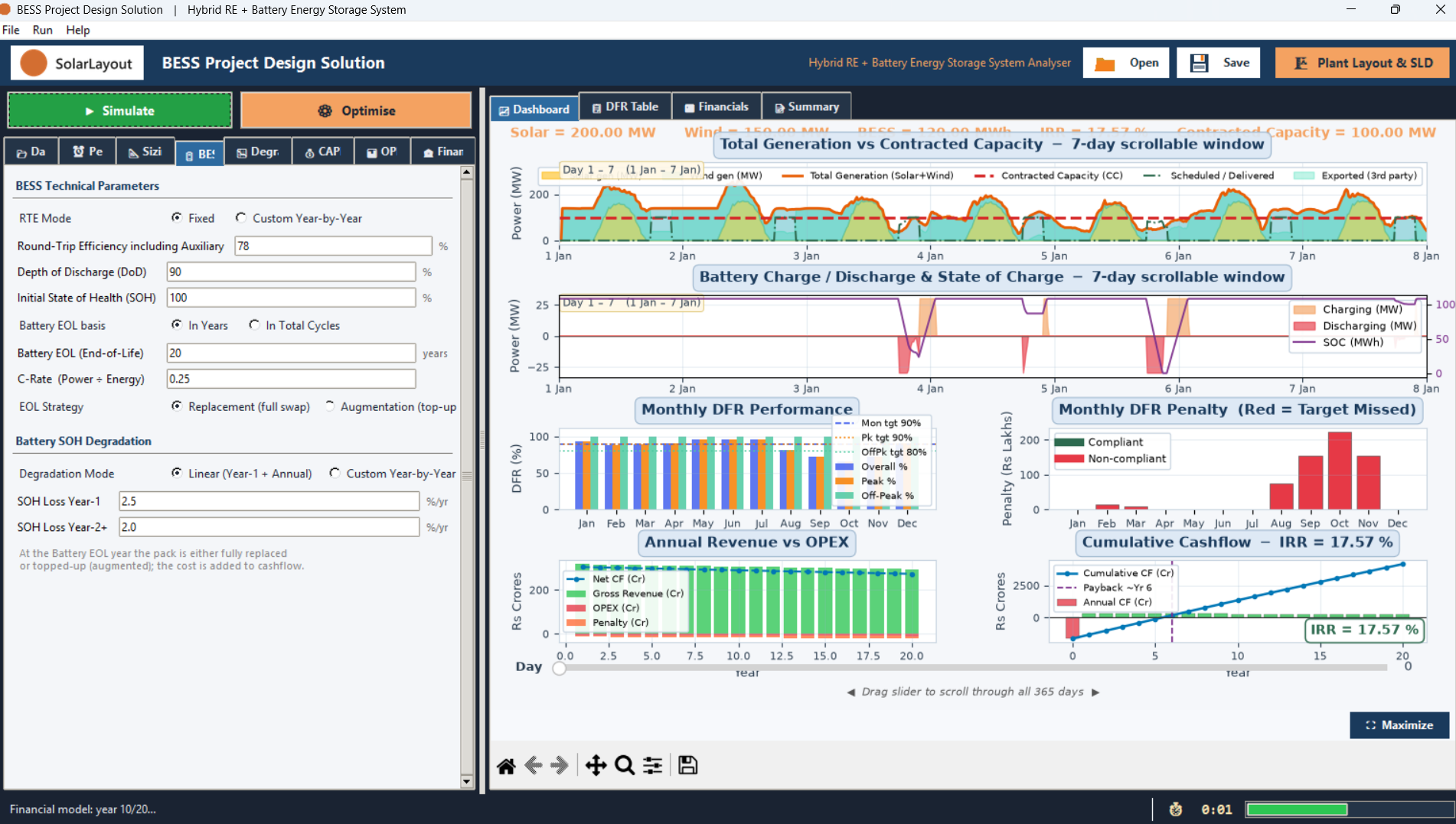
When it finishes, the status bar reads a single summary line giving the result's IRR, NPV and CAPEX, and the Solar, Wind and BESS sizing used, and the result notebook switches on its own to the 📈 Dashboard tab.
Read the Dashboard and Financials
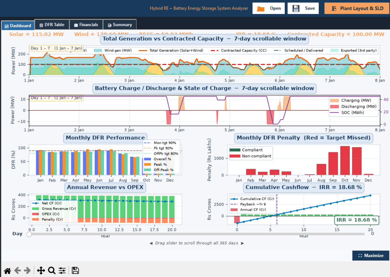
A header strip across the top of the 📈 Dashboard reports the sizing on the left — Solar, Wind and BESS capacity — and the headline IRR and Contracted Capacity on the right. Below it, six panels:
- Total Generation vs Contracted Capacity — a 7-day scrollable window of generation against the CC.
- Battery Charge / Discharge & State of Charge — the same window, with charge, discharge and state of charge; days with any grid charging are shaded.
- Monthly DFR Performance — Overall, Peak and Off-Peak DFR (Delivery Fulfilment Ratio — the share of the required energy actually delivered) against target, one group of bars per month.
- Monthly DFR Penalty — the shortfall penalty by month, red where a target was missed.
- Annual Revenue vs OPEX — revenue, operating cost and net cash flow, one point per project year.
- Cumulative Cashflow — annual and cumulative cash flow, with a payback marker and an IRR badge.
A Day slider beneath the first two panels scrolls both together across all 365 days.
The IRR badge on panel 6, and the equivalent tag on the 📝 Summary report, are coloured against a fixed 15% benchmark — not against the Project Target IRR field, under Optimisation Target on the 📊 OPEX tab. The two only agree when that field is left at its own default.
On the 💹 Financials tab, a headline line reports Total CAPEX, Project IRR and NPV, followed by LCOE (Levelised Cost of Energy) and LCOS (Levelised Cost of Storage) — the average cost per kWh delivered, and per kWh the battery itself handles — plus payback and the multiple on invested capital. Below the headline, a table runs one row per project year: degradation, delivered and exported energy, revenue, penalties, operating cost and cash flow.
Export a report
From the File menu, Export PDF Report… — or the same button on the 📝 Summary tab — writes a multi-page PDF covering the headline figures, the DFR result, the financial model and the dashboard charts. It needs this device activated, the same as Simulate.
The same menu offers a Word document, a plain-text report, a monthly DFR CSV, and a 15-minute time-series CSV of every dashboard series. To keep the session itself, use Save Project (.slb)… — it saves your inputs, the loaded generation data, the last result, and any Plant Layout or SLD drawing together. Open Project (.slb)… restores the inputs and the Plant Layout or SLD drawing from that file.